From Ray Casting to Ray Tracing with Python and VTK

In this post I will show how to use VTK to trace rays emanating from the cell-centers of a source mesh, intersecting with another target mesh, and then show you how to cast subsequent rays bouncing off the target adhering to physics laws. This will include calculating the cell-centers in a mesh, calculating the normal vectors at those cells, vector visualization through glyphs, as well as other elements of visualization like textures and scene-lighting.

---

Introduction

Background

In my last post, I used Python and VTK to show you how to perform ray-casting, i.e., intersection tests between arbitrary lines/rays and a mesh, and extraction of the intersection point coordinates through the vtkOBBTree class.

Today I’ll take the lessons learned about ray-casting with Python and VTK, and give you the tools to write your own ray-tracing algorithm using Python and VTK. Before proceeding, I strongly recommend that you read the ray-casting post, cause I will be re-using a lot of the functionality presented prior but I won’t repeat myself in too much detail.

Summary

We will start by creating the ‘environment’, i.e., the scene, which will comprise a yellowish half-sphere dubbed the sun, which will act as the ray-source, and a larger nicely textured sphere called earth which will be the target of those rays.

We will calculate the cell centers of the sun mesh and cast rays along the directions of the normal vector at each one of those cells. We will then use the vtkOBBTree functionality we presented in the last post about ray-casting to detect which of these rays intersect with earth, calculate the appropriate reflected vectors based on the earth normal vectors, and cast subsequent rays.

Now let me be clear, the code that will be presented today can not, by any stretch of the imagination, be called a fully-fledged ray-tracer. However, I will be presenting all necessary tools you would need to write your own ray-tracing algorithms using Python and VTK.

---

Ray-Tracing with Python & VTK

You can find the entire IPython Notebook I’ll be presenting today here. It contains a fair bit of code but it was structured in the same way as this post so you can easily look up the different parts of code and see what they do in detail.

Imports

As we’ve been doing in the past few posts we need to import vtk and numpy:

import vtk
import numpy

I know I’ve been saying it in nearly every post but here goes again: If for any reason you haven’t managed to get yourself a nice Python installation with ipython, numpy, and vtk, which are needed for this post, do yourselves a favor and use Anaconda as instructed in this previous post. Alternatively, you can opt for the Enthought Python Distribution (EPD) or Enthought Canopy. Of course there’s a truckload of other distros but I can vouch for the above and they all come with pre-compiled builds of VTK.

Helper-functions

The following ‘helper-functions’ are defined at the beginning of today’s notebook and used throughout:

• vtk_show(renderer, width=400, height=300): This function allows me to pass a vtkRenderer object and get a PNG image output of that render, compatible with the IPython Notebook cell output. This code was presented in this past post about VTK integration with an IPython Notebook.
• addLine(renderer, p1, p2, color=[0.0, 0.0, 1.0], opacity=1.0): This function uses vtk to add a line, defined by coordinates under p1 and p2, to a vtkRenderer object under renderer. In addition, it allows for the color and opacity level of the line to be defined and it was first presented in the previous post about ray-casting.
• addPoint(renderer, p, color=[0.0, 0.0, 0.0], radius=0.5): This function uses vtk to add a point-sized sphere (radius defaults to 0.5) defined by center coordinates under p. This function was first presented in the previous post about ray-casting, while similar code was detailed in this past post about VTK integration with an IPython Notebook.
• l2n = lambda l: numpy.array(l) and n2l = lambda n: list(n): These are just two simple lambda functions meant to quickly convert a list or tuple to a numpy.ndarray and vice-versa. The reason I wrote those, is that while VTK returns data like coordinates and vectors in tuple and list objects, which we need to ‘convert’ to numpy.ndarray objects in order to perform some basic vector math as we’ll see later on. In addition, we often need to feed such vectors and point back to VTK, so back-conversion is often necessary.

As you will see later we’re defining more ‘auxiliary functions’ which haven’t been presented prior to this post so we’re gonna be looking closely into what they do. The above ‘helper-functions’ all contain code that has been presented before at one time or another.

Options

As the code in today’s post deals with a lot of rendering and graphics-related parameters, I decided to set all these parameters as ‘options’ at the beginning of the notebook. You can change any of these and re-run the notebook to ascertain their effect.

You can see these options below but you do not have to pay too much attention to them right now. Apart from a few basic parameters defining attributes of the scene’s objects, they mostly deal with colors. In addition I will be referring back to these options later on while presenting the code.

# SUN OPTIONS
# Radius of the sun half-sphere
RadiusSun = 10.0
# Distance of sun's center from (0,0,0)
DistanceSun = 50.0
# Phi & Theta Resolution of sun
ResolutionSun = 6

# EARTH OPTIONS
# Radius of the earth sphere
RadiusEarth = 150.0
# Phi & Theta Resolution of earth
ResolutionEarth = 120

# RAY OPTIONS
# Length of rays cast from the sun. Since the rays we
# cast are finite lines we set a length appropriate to the scene.
# CAUTION: If your rays are too short they won't hit the earth 
# and ray-tracing won't be possible. Its better for the rays to be
# longer than necessary than the other way around
RayCastLength = 500.0

# COLOR OPTIONS
# Color of the sun half-sphere's surface
ColorSun = [1.0, 1.0, 0.0]
# Color of the sun half-sphere's edges
ColorSunEdge = [0.0, 0.0, 0.0]
# Color of the earth sphere's edges
ColorEarthEdge = [1.0, 1.0, 1.0]
# Background color of the scene
ColorBackground = [0.0, 0.0, 0.0]
# Ambient color light 
ColorLight = [1.0, 1.0, 0.0]
# Color of the sun's cell-center points
ColorSunPoints = [1.0, 1.0, 0.0]
# Color of the sun's cell-center normal-vector glyphs
ColorSunGlyphs = [1.0, 1.0, 0.0]
# Color of sun rays that intersect with earth
ColorRayHit = [1.0, 1.0, 0.0]
# Color of sun rays that miss the earth
ColorRayMiss = [1.0, 1.0, 1.0]
# Opacity of sun rays that miss the earth
OpacityRayMiss = 0.5
# Color of rays showing the normals from points on earth hit by sun rays
ColorEarthGlyphs = [0.0, 0.0, 1.0]
# Color of sun rays bouncing off earth 
ColorRayReflected = [1.0, 1.0, 0.0]

‘Environment’ Creation

We will start by creating the ‘environment’ within which we’ll perform our ray-tracing. This environment will comprise a half-sphere dubbed sun from which we will cast rays. Another sphere, which we will call earth, will receive and reflect those rays at appropriate angles.

Note that the sun and earth objects are by no means ‘in-scale’. Far from it actually (whole thing kinda looks like an earth-ball with a ceiling light above). I just named them as such to provide an apt analogy to what we’re doing here.

Create the sun

We start by creating the sun half-sphere through vtkSphereSource:

# Create and configure then sun half-sphere
sun = vtk.vtkSphereSource()
sun.SetCenter(0.0, DistanceSun, 0.0)
sun.SetRadius(RadiusSun)
sun.SetThetaResolution(ResolutionSun)
sun.SetPhiResolution(ResolutionSun)
sun.SetStartTheta(180)  # create a half-sphere

The source->mapper->actor process to create a sphere in VTK has been shown time after time and you can read about the mechanics in this previous post. However, I’ll go over a few novelties here. As you can see, upon creating a new vtkSphereSource under sun we set several parameters. The center coordinates and radius are defined through the DistanceSun and RadiusSun options discussed in the Options section.

What’s really important to note here is the theta and phi resolutions of the sun sphere set through the SetThetaResolution and SetPhiResolution methods respectively. VTK creates these spheres through the use of spherical coordinates and these resolution parameters define the number of points along the longitude and latitude directions respectively. A lower resolution will result in less points and therefore less triangles defining the sphere, making it look like something of a rough polygon.

However, as I mentioned in the Summary we will be casting a ray per triangle of the sun mesh. Hence, in order to keep the scene ‘clean’ and lower the computational cost, we set this resolutions to a mere 6 in the Options. Nonetheless, feel free to change this value in order to cast as many or as few rays as you wish. I’ll be showing the result of a resolution of 20 at the end of this post.

A last point I’d like to make is the usage of the SetStartTheta method. As I just said, VTK uses spherical coordinates to ‘design’ these spherical objects. Through the SetStartTheta, SetStopTheta, SetStartPhi, and SetStopPhi methods we define the starting and stopping angles (in degrees) for this sphere, allowing us to create spherical segments instead of a full sphere. In this example, and in the interest of keeping the scene ‘lean’ we’re only creating a ‘half-sphere’ through SetStartTheta(180).

With the vtkSphereSource defined and ‘stored’ under sun we simply create the appropriate vtkPolyDataMapper and vtkActor objects necessary to add this sphere to the scene:

# Create mapper
mapperSun = vtk.vtkPolyDataMapper()
mapperSun.SetInput(sun.GetOutput())

# Create actor
actorSun = vtk.vtkActor()
actorSun.SetMapper(mapperSun)
actorSun.GetProperty().SetColor(ColorSun)  #set color to yellow
actorSun.GetProperty().EdgeVisibilityOn()  # show edges/wireframe
actorSun.GetProperty().SetEdgeColor(ColorSunEdge)  #render edges as white

Once more, check this previous post to see what the deal with mappers and actors is in VTK. What I should mention here is that apart from using the GetProperty() method to access the properties of the actorSun object and set its color to ColorSun (set under Options), we also do so to enable the visibility of that mesh’s edges and set them to a color of ColorSunEdge. This way we’re visualizing the ‘wireframe’ of that object in order to see the individual mesh cells which come into play later.

Finally as we’ve done in all posts dealing with VTK we create a new vtkRenderer, add the actorSun object, set some camera properties, and use the vtk_show ‘helper-function’ to render the scene:

renderer = vtk.vtkRenderer()
renderer.AddActor(actorSun)
renderer.SetBackground(ColorBackground)

# Modify the camera with properties defined manually in ParaView
camera = renderer.MakeCamera()
camera.SetPosition(RadiusEarth, DistanceSun, RadiusEarth)
camera.SetFocalPoint(0.0, 0.0, 0.0)
camera.SetViewAngle(30.0)
renderer.SetActiveCamera(camera)

vtk_show(renderer, 600, 600)

Take a look at this past post about VTK integration with an IPython Notebook for an explanation of the vtkRenderer class, and the post about surface extraction to see what gives with the camera. What’s important to note is that we’ve created a vtkRenderer object under renderer to which we will continue adding new vtkActor objects as we go, thus enriching the scene.

The result of vtk_show can be seen in the following figure:

Here you can see the effect of that ‘resolution’ stuff I was talking about before. The sun half-sphere is jagged and rough. Nonetheless, it still comprises plenty of cells and therefore ray-sources for our example.

Create the earth

Let’s go onto creating earth. As during my posts I’ve showed you how to create spheres a trillion times I thought I’d kick it up a notch and show you how to texture one, giving it a bit of razzle-dazzle :). We start by creating a new sphere under earth as such:

# Create and configure the earth sphere
earth = vtk.vtkSphereSource()
earth.SetCenter(0.0, -RadiusEarth, 0.0)
earth.SetThetaResolution(ResolutionEarth)
earth.SetPhiResolution(ResolutionEarth)
earth.SetRadius(RadiusEarth)

Typical stuff as you can see, just keep in mind that the earth variable holds the pointer to the, now configured, vtkSphereSource object. You’ll also note that all parameters are set to values defined in the Options section so take a look if you will.

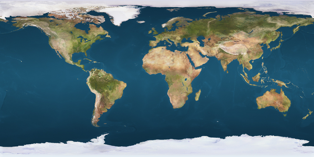
Now let’s move on to texturing. I used a texture of the earth I downloaded as a JPEG file from http://planetpixelemporium.com/download/download.php?earthmap1k.jpg and placed along this post’s notebook. Alternatively, you can download it from the blog repository under here. Firstly, we need to load that image as such:

# Load a JPEG file with an 'earth' texture downloaded from the above link
reader = vtk.vtkJPEGReader()
reader.SetFileName("earthmap1k.jpg")
reader.Update()

All we do is use the vtkJPEGReader class to create reader, set the filename, and read in the image through Update.

I want to specify, that as the reader is not used directly but is rather a part of the VTK pipeline, we don’t really need to call Update. That method will be called by subsequent objects that use reader as an input. However, while debugging VTK code, progressively updating the pipeline allows us to verify which part of the pipeline didn’t work instead of getting an arbitrary error at some point down the road.

Next, we create the actual texture:

# Create a new 'vtkTexture' and set the loaded JPEG
texture = vtk.vtkTexture()
texture.SetInputConnection(reader.GetOutputPort())
texture.Update()

Here we create a new vtkTexture object and, using the SetInputConnection and GetOutputPort methods, connect its input to the output of the reader object holding the texture image.

So far so good right? What needs to be done now to complete the texturing, is to map this texture to our earth sphere. Now this might be a tad confusing so I’ll break it down:

# Map the earth texture to the earth sphere
map_to_sphere = vtk.vtkTextureMapToSphere()
map_to_sphere.SetInputConnection(earth.GetOutputPort())
map_to_sphere.PreventSeamOn()
texture.Update()

As a first step we create a new vtkTextureMapToSphere object under map_to_sphere which “generates 2D texture coordinates by mapping input dataset points onto a sphere”. Check the code carefully, and you’ll realize we’re not connecting map_to_sphere with texture but only with earth! This class will just calculate the coordinates based on the earth sphere but does not set a texture yet (that occurs later).

And now for the finishing touches:

# Create a new mapper with the mapped texture and sphere
mapperEarth = vtk.vtkPolyDataMapper()
mapperEarth.SetInputConnection(map_to_sphere.GetOutputPort())

# Create actor
actorEarth = vtk.vtkActor()
actorEarth.SetMapper(mapperEarth)
actorEarth.SetTexture(texture)
actorEarth.GetProperty().EdgeVisibilityOn()  # show edges/wireframe
actorEarth.GetProperty().SetEdgeColor(ColorEarthEdge)  #render edges as white

renderer.AddActor(actorEarth)
vtk_show(renderer, 600, 600)

You should be familiar with the vtkPolyDataMapper and vtkActor classes so I won’t repeat myself. What you should pay attention to is that instead of using earth as a source for mapperEarth we instead use map_to_sphere which contains the vtkTextureMapToSphere object we just saw! In addition, upon creating actorEarth we finally set the texture through actorEarth.SetTexture(texture). As you can see the texture goes straight into the appropriate vtkActor object, which along with the texture-mapping provides us with a nicely textured sphere.

Finally, we make the earth wireframe visible with a ColorEarthEdge color, add actorEarth to renderer, and use vtk_show to render the scene resulting in the following figure:

Adding lighting to the scene

Now you might say “what gives? we went to so much trouble to texture that stupid ball and it looks all dark and crummy!”. Well at least I obviously thought so, thus I decided to shed a little light on the situation (I know, stupidest pun ever).

Before I continue, I want to mention that all VTK scenes comes with a default ‘headlight’ which follows the camera and illuminates the scene. In most cases that’s enough to see our rendering but often we need a lil’ extra.

In this case I added a light point-source through the vtkLight class. Let’s see how that was done:

# Create a new vtkLight
light = vtk.vtkLight()
# Set its ambient color to yellow
light.SetAmbientColor(ColorLight)
# Set a 180 degree cone angle to avoid a spotlight-effect
light.SetConeAngle(180)
# Set its position to the sun's center
light.SetPosition(sun.GetCenter())
# Set its focal-point to the earth's center 
light.SetFocalPoint(earth.GetCenter())
# Set it as part of the scene (positional) and not following the camera
light.SetPositional(True)
renderer.AddLight(light)

vtk_show(renderer, 600, 600)

Initially, we create a vtkLight object under light, and set an appropriate ColorLight which was defined at the Options section. As you can see I set the position of the light-source to the center of the sun half-sphere, which just makes sense (you know, sun and all that), through light.SetPosition(sun.GetCenter()), while its focal point is the center of the earth sphere.

What’s important to note here is that these lights are typically ‘spotlights’ adding a ‘narrow’ beam of light to the scene. By using SetConeAngle(180) we create a uniform semi-spherical light that evenly illuminates the entire scene residing beneath the center of the sun half-sphere. Lastly, please pay attention to the SetPositional(True) method which makes this light a constant part of the scene, forcing it in place, and not allowing it to move with respect to the scene’s camera.

After adding light to the renderer, we once more use vtk_show to render the scene and get this figure (makes quite the difference right?):

‘Prepare’ the Sun Rays

As I said in the Summary, we will be casting rays from each cell-center of the sun mesh following the direction of the normal vectors of those cells. Naturally, we first need to calculate these quantities, thus ‘defining’ the rays.

Calculate the cell-centers of the sun half-sphere

Firstly, we need to calculate the coordinates at the center of each cell on the sun mesh. Thankfully VTK provides us with a nifty class called vtkCellCenters to do so:

cellCenterCalcSun = vtk.vtkCellCenters()
cellCenterCalcSun.SetInput(sun.GetOutput())
cellCenterCalcSun.Update()

As you can see this is as simple as VKT gets. We merely create a vtkCellCenters object under cellCenterCalcSun, and connect its input with sun.GetOutput(). Upon using Update, the calculation is complete.

Now let us visualize those points using the addPoint and vtk_show helper functions:

# Get the point centers from 'cellCenterCalc'
pointsCellCentersSun = cellCenterCalcSun.GetOutput(0)

# Loop through all point centers and add a point-actor through 'addPoint'
for idx in range(pointsCellCentersSun.GetNumberOfPoints()):
    addPoint(renderer, pointsCellCentersSun.GetPoint(idx), ColorSunPoints)

vtk_show(renderer, 600, 600)

We first ‘extract’ the cell-centers through cellCenterCalcSun.GetOutput(0), storing the result of vtkPoints type under pointsCellCentersSun. Subsequently, we loop through these points and use addPoint to add them to the vtkRenderer object we created before and which now resides under renderer. Note that we’re looping using the range built-in and the GetNumberOfPoints() method to get the total number of points found. The resulting figure can then be seen below.

Calculate normal vectors at the center of each cell

Now that we have the cell-centers, which will act as the ‘source points’ of the sun rays, we need to calculate the normal vectors at those points which will define the directions of the rays. Once more, VTK provides the tools but doesn’t make it easy or clear for us (you wouldn’t appreciate it working if it was easy, would you now 🙂 ?). Let’s see how it’s done:

# Create a new 'vtkPolyDataNormals' and connect to the 'sun' half-sphere
normalsCalcSun = vtk.vtkPolyDataNormals()
normalsCalcSun.SetInputConnection(sun.GetOutputPort())

# Disable normal calculation at cell vertices
normalsCalcSun.ComputePointNormalsOff()
# Enable normal calculation at cell centers
normalsCalcSun.ComputeCellNormalsOn()
# Disable splitting of sharp edges
normalsCalcSun.SplittingOff()
# Disable global flipping of normal orientation
normalsCalcSun.FlipNormalsOff()
# Enable automatic determination of correct normal orientation
normalsCalcSun.AutoOrientNormalsOn()
# Perform calculation
normalsCalcSun.Update()

So we start by creating a new vtkPolyDataNormals object under normalsCalcSun (remember this variable name, we’ll be using it lots later on). We then ‘connect’ this object to the sun mesh where we want those normals to be calculated.

The rest boils down to configuring the vtkPolyDataNormals class to give us what we want. You can see what each call does in the comments above but I should stress a few points here. vtkPolyDataNormals can calculate the normal vectors at the mesh points and/or cells. However, we only want the latter, so we turn off calculation at points with ComputePointNormalsOff() and only enable calculation at cells with ComputeCellNormalsOn().

Subsequently, we turn ‘splitting’ off through SplittingOff(). First of all that only makes sense when calculating point-normals. What it would do is ‘split’, thus create, multiple normals at points belonging to cells with very sharp edges, i.e., steep angles between cells. However, we only want cell normals so we don’t care about it too much.

We then want to make sure that the normals have a correct orientation, i.e., that they would be ‘pointing’ outwards and not towards the center of the sun half-sphere. To ensure that, we first disable global flipping through ‘FlipNormalsOff()’, and we enable automatic orientation determination through AutoOrientNormalsOn(). Now this last call is a god-send as it will make sure the normals point outwards which we sorely need to correctly cast our rays.

However, I want to point you to the vtkPolyDataNormals docs, and in particular the docstring for the AutoOrientNormalsOn method which reads: “Turn on/off the automatic determination of correct normal orientation. NOTE: This assumes a completely closed surface (i.e. no boundary edges) and no non-manifold edges. If these constraints do not hold, all bets are off. This option adds some computational complexity, and is useful if you don’t want to have to inspect the rendered image to determine whether to turn on the FlipNormals flag. However, this flag can work with the FlipNormals flag, and if both are set, all the normals in the output will point ”inward“.”

What that means is that while AutoOrientNormalsOn is crazy-useful to ensure correct orientation, it comes with stringent requirements, and its not always guaranteed to succeed. Thankfully, our sun mesh fits these criteria and calling Update() completes the calculation.

Visualize normal vectors at the cell-centers of sun’s surface as glyphs

Before proceeding on to casting and tracing the sun rays we will visualize the normal vectors calculated on the sun mesh as glyphs using the vtkGlyph3D class.

Before I show you the code lets take a look at the docstring of the vtkGlyph3D class: “vtkGlyph3D is a filter that copies a geometric representation (called a glyph) to every point in the input dataset. The glyph is defined with polygonal data from a source filter input. The glyph may be oriented along the input vectors or normals, and it may be scaled according to scalar data or vector magnitude”.

What we’re going to do here, is create a single arrow through the vtkArrowSource class and use it as a glyph. Then we’ll use the normal vectors we calculated before, and which are stored under normalsCalcSun, to place and orient those glyphs. Let’s inspect the code:

# Create a 'dummy' 'vtkCellCenters' to force the glyphs to the cell-centers
dummy_cellCenterCalcSun = vtk.vtkCellCenters()
dummy_cellCenterCalcSun.VertexCellsOn()
dummy_cellCenterCalcSun.SetInputConnection(normalsCalcSun.GetOutputPort())

# Create a new 'default' arrow to use as a glyph
arrow = vtk.vtkArrowSource()

# Create a new 'vtkGlyph3D'
glyphSun = vtk.vtkGlyph3D()
# Set its 'input' as the cell-center normals calculated at the sun's cells
glyphSun.SetInputConnection(dummy_cellCenterCalcSun.GetOutputPort())
# Set its 'source', i.e., the glyph object, as the 'arrow'
glyphSun.SetSourceConnection(arrow.GetOutputPort())
# Enforce usage of normals for orientation
glyphSun.SetVectorModeToUseNormal()
# Set scale for the arrow object
glyphSun.SetScaleFactor(5)

# Create a mapper for all the arrow-glyphs
glyphMapperSun = vtk.vtkPolyDataMapper()
glyphMapperSun.SetInputConnection(glyphSun.GetOutputPort())

# Create an actor for the arrow-glyphs
glyphActorSun = vtk.vtkActor()
glyphActorSun.SetMapper(glyphMapperSun)
glyphActorSun.GetProperty().SetColor(ColorSunGlyphs)
# Add actor
renderer.AddActor(glyphActorSun)

vtk_show(renderer, 600, 600)

Now this code is a little convoluted so I’ll break it down. The first very important thing to mention is that we do not simply use the normals calculated beforehand stored within normalsCalcSun. As you can see in the first lines of the snippet above, we feed those normals to a ‘dummy’ vtkCellCenters called dummy_cellCenterCalcSun. This forces the glyphs to be placed on the cell-centers of the sun mesh.

Subsequently, we create the glyphs. Note that we first create arrow, a vtkArrowSource object representing a default arrow, which we will use as the ‘base’ glyph. Now this glyph can be any ‘source’ class, e.g. a cone through the vtkConeSource class, a sphere through the vtkSphereSource class, etc etc. The only reason I chose an arrow was cause it nicely shows the direction the sun rays will follow.

We then create a new vtkGlyph3D object under glyphSun. The important thing to note here is the difference between the SetInputConnection and SetSourceConnection methods. The latter just connects to the ‘source’ glyph, i.e., the arrow in our case. The SetInputConnection call is given dummy_cellCenterCalcSun.GetOutputPort(), i.e., the normal vectors calculated and then positioned at the cell-centers of the sun mesh.

Henceforth things are simple: we enforce orientation of the created glyphs to the supplied normal vectors through SetVectorModeToUseNormal(), and we provide a ‘scale factor’ for the base glyphs, which will just uniformly scale the arrow and its default size. The rest has been shown a thousand times: we create a vtkPolyDataMapper to map the create object to graphics primitives and connect to the glyphSun output. We then create a standard vtkActor, connect to the aforementioned mapper, and use its GetProperty() method to SetColor(ColorSunGlyphs).

Finally, using the vtk_show helper-function yields the following figure. As you can see we have visualized all normal vectors with arrows, showing the direction our sun rays will follow.

Prepare for ray-tracing

We’re finally getting to the ray-tracing part of the post. All we now need to do is prepare the vtkOBBTree object for earth as I showed in the last post on ray-casting. If you haven’t read it then I strongly recommend that you do now cause I won’t explain the details again.

Firstly, we create a new vtkOBBTree object with the earth mesh where we’re going to test for intersection with rays coming from the sun. This is done as simply as this:

obbEarth = vtk.vtkOBBTree()
obbEarth.SetDataSet(earth.GetOutput())
obbEarth.BuildLocator()

Just keep obbEarth in mind cause we’ll be using extensively to test for intersections later.

Then we need calculate the normal vectors at all cell-centers on the earth mesh as we’re going to need that information to cast reflected rays. The process here is exactly the same as the one we used to calculate the normal vectors for the sun mesh:

# Create a new 'vtkPolyDataNormals' and connect to the 'earth' sphere
normalsCalcEarth = vtk.vtkPolyDataNormals()
normalsCalcEarth.SetInputConnection(earth.GetOutputPort())

# Disable normal calculation at cell vertices
normalsCalcEarth.ComputePointNormalsOff()
# Enable normal calculation at cell centers
normalsCalcEarth.ComputeCellNormalsOn()
# Disable splitting of sharp edges
normalsCalcEarth.SplittingOff()
# Disable global flipping of normal orientation
normalsCalcEarth.FlipNormalsOff()
# Enable automatic determination of correct normal orientation
normalsCalcEarth.AutoOrientNormalsOn()
# Perform calculation
normalsCalcEarth.Update()

Just remember that normalsCalcEarth now holds the normal vectors for the earth mesh.

Finally, we define two ‘auxiliary-functions’ to nicely wrap the intersection testing functionality offered by the vtkOBBTree class:

def isHit(obbTree, pSource, pTarget):
    r"""Returns True if the line intersects with the mesh in 'obbTree'"""
    code = obbTree.IntersectWithLine(pSource, pTarget, None, None)
    if code==0:
        return False
    return True

def GetIntersect(obbTree, pSource, pTarget):
    
    # Create an empty 'vtkPoints' object to store the intersection point coordinates
    points = vtk.vtkPoints()
    # Create an empty 'vtkIdList' object to store the ids of the cells that intersect
    # with the cast rays
    cellIds = vtk.vtkIdList()
    
    # Perform intersection
    code = obbTree.IntersectWithLine(pSource, pTarget, points, cellIds)
    
    # Get point-data 
    pointData = points.GetData()
    # Get number of intersection points found
    noPoints = pointData.GetNumberOfTuples()
    # Get number of intersected cell ids
    noIds = cellIds.GetNumberOfIds()
    
    assert (noPoints == noIds)
    
    # Loop through the found points and cells and store
    # them in lists
    pointsInter = []
    cellIdsInter = []
    for idx in range(noPoints):
        pointsInter.append(pointData.GetTuple3(idx))
        cellIdsInter.append(cellIds.GetId(idx))
    
    return pointsInter, cellIdsInter

Again, if you haven’t read the last post on ray-casting, do so and the above will make complete sense to you.

The isHit function will simply return True or False depending on whether a given ray intersects with obbTree, which in our case will only be obbEarth.

The second function is a little more complex but the mechanics were detailed in the previous post. I’ve included comments in the code so you can get what it does but I’m not going to spoon-feed this to you again. Read up :).

In a nutshell it will return two list objects pointsInter and cellIdsInter. The former will contain a series of tuple objects with the coordinates of the intersection points. The latter will contain the ‘id’ of the mesh cells that were ‘hit’ by that ray. This information is vital as through these ids we’ll be able to get the correct normal vector for that earth cell and calculate the appropriate reflected vector as we’ll see below.

Perform ray-casting operations and visualize different aspects

Finally the moment you’ve all been waiting for! The ray-tracing! Now since the code to perform the whole operation is too much to explain in a single go, I decided to repeat the process three times, visualizing and explaining different aspects of it every time.

Cast rays, test for intersections, and visualize the rays that hit earth

In this first step we will only cast the rays from the sun, test for their intersection, or lack thereof, and render the rays that do hit the earth with a different color than the ones that miss it. In addition, we’ll also render points at those intersection points as they will be the ‘source’ points for the reflected rays later on.

The code is the following:

# Extract the normal-vector data at the sun's cells
normalsSun = normalsCalcSun.GetOutput().GetCellData().GetNormals()

# Loop through all of sun's cell-centers
for idx in range(pointsCellCentersSun.GetNumberOfPoints()):
    # Get coordinates of sun's cell center
    pointSun = pointsCellCentersSun.GetPoint(idx)
    # Get normal vector at that cell
    normalSun = normalsSun.GetTuple(idx)
    
    # Calculate the 'target' of the ray based on 'RayCastLength'
    pointRayTarget = n2l(l2n(pointSun) + RayCastLength*l2n(normalSun))
    
    # Check if there are any intersections for the given ray
    if isHit(obbEarth, pointSun, pointRayTarget):  # intersections were found
        # Retrieve coordinates of intersection points and intersected cell ids
        pointsInter, cellIdsInter = GetIntersect(obbEarth, pointSun, pointRayTarget)
        # Render lines/rays emanating from the sun. Rays that intersect are
        # rendered with a 'ColorRayHit' color
        addLine(renderer, pointSun, pointsInter[0], ColorRayHit)
        # Render intersection points
        addPoint(renderer, pointsInter[0], ColorRayHit)
    else:
        # Rays that miss the earth are rendered with a 'ColorRayMiss' colors
        # and a 25% opacity
        addLine(renderer, pointSun, pointRayTarget, ColorRayMiss, opacity=0.25)
        
vtk_show(renderer, 600, 600)

As you no doubt remember, cause you’ve been paying attention all this time, the normalsCalcSun is a vtkPolyDataNormals object which holds the normal vectors calculated at the cell-centers of the sun mesh. As you can see from the 1st line of the code, retrieving the actual normal vector data is easy but not intuitive. First we get all output out through GetOutput. However, the output could have point-data and/or cell-data depending on how we configured the class. In our case we want the cell-data which we retrieve through GetCellData() followed by GetNormals() which will give a set of normal vectors under normalsSun.

Afterwards, as we want to cast a ray from every cell-center on the sun mesh, we loop through these points stored under pointsCellCentersSun. The idx variable will hold an index to that point.

We store the coordinates of each such point under pointSun through pointsCellCentersSun.GetPoint(idx), while we store the corresponding normal vector under normalSun through normalsSun.GetTuple(idx). Now we have the ‘source’ point and direction our ray should follow.

In our example, however, rays are merely lines of finite length. Due to that we have to define a ‘target’ point which we want to make sure it won’t miss the earth due to an insufficient length. To that end I’ve defined a variable RayCastLength under the Options, which naturally will define the length of the ‘ray’. As such we use the following line (repeating it here) to calculate the coordinates of the ‘target’ point:

pointRayTarget = n2l(l2n(pointSun) + RayCastLength*l2n(normalSun))

Note that we use the n2l and l2n helper-functions to quickly convert a list or tuple object as retrieved from VTK, into a numpy.ndarray object and vice-versa. As I mentioned in the Helper-Functions section, this conversion allows us to use numpy and perform some basic vector-math, which in this case is vector addition and multiplication.

Now we finally have all we need to cast that pesky ray, i.e. the ‘source’ and ‘target’ coordinates! We first use the isHit auxiliary-function to cast that ray and see if it intersects with earth as such:

isHit(obbEarth, pointSun, pointRayTarget)

If we get a False back then the ray does not intersect and its not worth processing further but we render it anyway through addLine with a ColorRayMiss color, and a 25% opacity (in our case resulting in a faded whitish ray).

However, should the ray intersect with earth then its worth processing. We then re-cast that ray and retrieve the intersection point coordinates and ids of the earth cells the ray hit through the GetIntersect auxiliary-function we defined before (repeating the line here):

pointsInter, cellIdsInter = GetIntersect(obbEarth, pointSun, pointRayTarget)

As I explained before, the pointsInter variable now holds a list of tuple objects with the coordinates of each intersection point in order. The cellIdsInter contains simple int entries with the id of the mesh cells that were this but we won’t use that information in this step. What we will however use is pointsInter[0], i.e., the 1st point that was hit by the ray.

We consider the earth to be a reflective body so we don’t care about the following intersection points as the rays that impinge on earth are supposed to be reflected entirely.

The rest is super-simple. We just use addLine and addPoint to render the ray that hits the earth and the 1st intersection point, which under default Options should appear as yellow.

After looping through all cell-centers in the sun, cast those rays, and define whether they hit or miss, we finally call vtk_show and end up with the next figure.

Visualize the normal vectors at the cells where sun’s rays intersect with earth

During this next step we’ll add a lil’ more complexity, and visualize the earth normal vectors at the points where rays from the sun intersect and we’ll do so again through glyphs. However, unlike the case where we rendered all normals on the sun surface, here we only want to render the normals at points were intersections were detected. Thus, the glyph process is slightly different and allows for more flexibility.

# Extract the normal-vector data at the sun's cells
normalsSun = normalsCalcSun.GetOutput().GetCellData().GetNormals()
# Extract the normal-vector data at the earth's cells
normalsEarth = normalsCalcEarth.GetOutput().GetCellData().GetNormals()

# Create a dummy 'vtkPoints' to act as a container for the point coordinates
# where intersections are found
dummy_points = vtk.vtkPoints()
# Create a dummy 'vtkDoubleArray' to act as a container for the normal
# vectors where intersections are found
dummy_vectors = vtk.vtkDoubleArray()
dummy_vectors.SetNumberOfComponents(3)
# Create a dummy 'vtkPolyData' to store points and normals
dummy_polydata = vtk.vtkPolyData()

# Loop through all of sun's cell-centers
for idx in range(pointsCellCentersSun.GetNumberOfPoints()):
    # Get coordinates of sun's cell center
    pointSun = pointsCellCentersSun.GetPoint(idx)
    # Get normal vector at that cell
    normalSun = normalsSun.GetTuple(idx)

    # Calculate the 'target' of the ray based on 'RayCastLength'
    pointRayTarget = n2l(l2n(pointSun) + RayCastLength*l2n(normalSun))
    
    # Check if there are any intersections for the given ray
    if isHit(obbEarth, pointSun, pointRayTarget):
        # Retrieve coordinates of intersection points and intersected cell ids
        pointsInter, cellIdsInter = GetIntersect(obbEarth, pointSun, pointRayTarget)
        # Get the normal vector at the earth cell that intersected with the ray
        normalEarth = normalsEarth.GetTuple(cellIdsInter[0])
        
        # Insert the coordinates of the intersection point in the dummy container
        dummy_points.InsertNextPoint(pointsInter[0])
        # Insert the normal vector of the intersection cell in the dummy container
        dummy_vectors.InsertNextTuple(normalEarth)

# Assign the dummy points to the dummy polydata
dummy_polydata.SetPoints(dummy_points)
# Assign the dummy vectors to the dummy polydata
dummy_polydata.GetPointData().SetNormals(dummy_vectors)
        
# Visualize normals as done previously but using 
# the 'dummyPolyData'
arrow = vtk.vtkArrowSource()

glyphEarth = vtk.vtkGlyph3D()
glyphEarth.SetInput(dummy_polydata)
glyphEarth.SetSourceConnection(arrow.GetOutputPort())
glyphEarth.SetVectorModeToUseNormal()
glyphEarth.SetScaleFactor(5)

glyphMapperEarth = vtk.vtkPolyDataMapper()
glyphMapperEarth.SetInputConnection(glyphEarth.GetOutputPort())

glyphActorEarth = vtk.vtkActor()
glyphActorEarth.SetMapper(glyphMapperEarth)
glyphActorEarth.GetProperty().SetColor(ColorEarthGlyphs)

renderer.AddActor(glyphActorEarth)

vtk_show(renderer, 600, 600)

Firstly, we extract the normal vectors for the sun and earth, much as we did before, and store them under normalsSun and normalsEarth respectively.

Then, we create two ‘dummy’ containers that will store the intersection point coordinates (dummy_points) and the earth normals (dummy_vectors) where sun rays intersected. We will use this information to render those, and only those, normals on earth. Note that dummy_points is of type vtkPoints, while dummy_vectors is of vtkDoubleArray type. We ‘configure’ dummy_vectors to have 3 components through SetNumberOfComponents which are going to be the vector’s x, y, and z, components. Finally, we define dummy_polydata of type vtkPolyData, which will ‘house’ the ‘dummy’ points and vectors and which we will pass to the vtkGlyph3D class later on.

The loop in this step is very similar to the one we presented in the previous step. We simply go through all cell-centers on the sun mesh, cast-rays, and test for their intersection. The key difference is that instead of rendering rays, we now use the cellIdsInter to get the cell id of the 1st cell, i.e., the cell the sun ray first intersects with. We then use that id to retrieve the normal vector on the earth where the ray hit as such:

normalEarth = normalsEarth.GetTuple(cellIdsInter[0])

Subsequently, we use the InsertNextPoint and InsertNextTuple methods to ‘push’ the retrieved point coordinates and normal vectors into the dummy containers. Once the loop is complete, we set those points and vectors to the dummy_polydata container as points and normals. We do this through the SetPoints and GetPointData().SetNormals() methods respectively.

The rest is mostly the same as the previous glyph rendering we did for the sun normals. The only difference is that the source of the glyphEarth object is now the dummy_polydata object we just composed. As you can understand, this approach allowed us to render fully-customized glyphs. The result of this step can be seen in the next figure where we can now see the earth normal vectors where sun rays intersect.

Calculate and visualize reflected rays

Here comes the final step. We now have all information we need to cast rays from the sun, detect which ones hit earth, and use vector math to cast subsequent rays that are reflected off the earth surface with the appropriate orientation.

We first define a little ‘auxiliary-function’ called calcVecR that calculates a reflected vector from the incident and normal vectors:

def calcVecR(vecInc, vecNor):
    vecInc = l2n(vecInc)
    vecNor = l2n(vecNor)
    
    vecRef = vecInc - 2*numpy.dot(vecInc, vecNor)*vecNor
    
    return n2l(vecRef)

As you can see we use the l2n and n2l helper-functions to quickly convert vectors from list or tuple objects to numpy.ndarray objects and vice-versa. A nice article detailing this type of vector math used in ray-tracing can be seen here.

Finally, we repeat the whole process we saw before but this time we only calculate and render the reflected rays:

# Extract the normal-vector data at the sun's cells
normalsSun = normalsCalcSun.GetOutput().GetCellData().GetNormals()
# Extract the normal-vector data at the earth's cells
normalsEarth = normalsCalcEarth.GetOutput().GetCellData().GetNormals()

# Loop through all of sun's cell-centers
for idx in range(pointsCellCentersSun.GetNumberOfPoints()):
    # Get coordinates of sun's cell center
    pointSun = pointsCellCentersSun.GetPoint(idx)
    # Get normal vector at that cell
    normalSun = normalsSun.GetTuple(idx)
    
    # Calculate the 'target' of the ray based on 'RayCastLength'
    pointRayTarget = n2l(l2n(pointSun) + RayCastLength*l2n(normalSun))
    
    # Check if there are any intersections for the given ray
    if isHit(obbEarth, pointSun, pointRayTarget):
        # Retrieve coordinates of intersection points and intersected cell ids
        pointsInter, cellIdsInter = GetIntersect(obbEarth, pointSun, pointRayTarget)
        # Get the normal vector at the earth cell that intersected with the ray
        normalEarth = normalsEarth.GetTuple(cellIdsInter[0])
        
        # Calculate the incident ray vector
        vecInc = n2l(l2n(pointRayTarget) - l2n(pointSun))
        # Calculate the reflected ray vector
        vecRef = calcVecR(vecInc, normalEarth)
        
        # Calculate the 'target' of the reflected ray based on 'RayCastLength'
        pointRayReflectedTarget = n2l(l2n(pointsInter[0]) + RayCastLength*l2n(vecRef))

        # Render lines/rays bouncing off earth with a 'ColorRayReflected' color
        addLine(renderer, pointsInter[0], pointRayReflectedTarget, ColorRayReflected)
        
vtk_show(renderer, 600, 600)

The only ‘new’ lines here to which you should pay attention, reside within the loop and are the following:

# Calculate the incident ray vector
vecInc = n2l(l2n(pointRayTarget) - l2n(pointSun))
# Calculate the reflected ray vector
vecRef = calcVecR(vecInc, normalEarth)
        
# Calculate the 'target' of the reflected ray based on 'RayCastLength'
pointRayReflectedTarget = n2l(l2n(pointsInter[0]) + RayCastLength*l2n(vecRef))

As you can see, we just calculate the vector of the incident ray, a ray which we know hits the earth, by subtracting the coordinates of the ray’s ‘target’ point on earth from the ray’s ‘source’ point on the sun.

Then we use the simple auxiliary-function calcVecR to calculate the vector of the reflected ray through vecRef = calcVecR(vecInc, normalEarth). Finally we calculate a ‘target’ point for this reflected ray, much as we did when we first cast the rays from the sun, as such:

pointRayReflectedTarget = n2l(l2n(pointsInter[0]) + RayCastLength*l2n(vecRef))

At long last, we just render these reflected rays through addLine and vtk_show and get the next figure.

---

Outro

As you can see, we just went through all the necessary components to perform ray-tracing with a given ‘source’ object being the sun, and a ‘target’ object being the earth. For a full ray-tracer, one would need to perform this sort of calculations and tests for each ‘target’ object and keep casting rays. In a more realistic ray-tracer two additional concepts would have to be accounted for:

• Each ray would need to carry a certain amount of ‘energy’ which would gradually deplete, eventually running out, thus providing a means of terminating an otherwise endless loop.
• The ‘target’ object would not merely reflect the impinging rays but part of the ray’s energy would be reflected while the rest would refract through the ‘target’ object. Therefore, every ray-hit would actually result in two subsequent rays that would need to be cast and traced. However, that would require our different objects to exhibit ‘material’ characteristics, thus defining the reflective and refractive indices as well as attenuation that would further deplete the ray’s energy as it passes through such an object.

However, the above would result in code that too much for a conceptual post and I’ll leave it up to you to extend it for yourselves. I just hope I’ve provided you with all you needed to know to realize something of the sort.

One last thing before I close. I mentioned in the beginning of this post, such a long time ago, that we needed to have a low ‘resolution’ for the sun mesh in order to get a small number of triangles, and therefore rays. If we had a very refined mesh on the sun not only would we significantly increase the number of rays, and therefore boggle the graphics, but we’d also be faced with quite a bit of computational weight. Regardless, here’s the final render showing the entire scene if we were to set the ResolutionSun variable under Options from its default value of 6 to a value of 20.

Pretty gorgeous albeit messy, wouldn’t you say 🙂 ?

Links & Resources

Material

Here’s the material used in this post:

• IPython Notebook showing the entire process.
• Earth Texture.
• Reflections and Refractions in Ray-Tracing by Bram de Greve: Article explaining the math and physics used in ray-tracing.

Check these past posts which were used and referenced today:

• Anaconda: The crème de la crème of Python distros
• IPython Notebook & VTK
• Surface Extraction: Creating a mesh from pixel-data using Python and VTK
• Ray Casting with Python and VTK: Intersecting lines/rays with surface meshes

Don’t forget: all material I’m presenting in this blog can be found under the PyScience BitBucket repository.

---

I hope you enjoyed going through this post as much as I enjoyed putting it together. This was by far my longest post yet, and it took a preposterous amount of my free time to prepare, but I hope I managed to introduce you to a large variety of different VTK classes which you can utilize in a gazillion of different ways.

I’ve tested the accompanying notebook on Mac OS X 10.9.5, Windows 8.1, and Linux Mint 17, all running the latest Anaconda Python with a py27 environment as discussed in my first post. Thus, I have no reason to believe that you’ll run into trouble but if you do then you know the drill (comment here and I’ll get back to you) :).

One last quick note: I know I never mentioned it before, cause – to my dismay – I tend to consider a few things as common knowledge, but VTK has not yet been wrapped for Python 3 even though the porting has been in the works for some time. For better or for worse, Python+VTK code will need to be executed on Python 2 for the time being :).