Multi-Modal Image Segmentation with Python & SimpleITK

In this post I will show how to use SimpleITK to perform multi-modal segmentation on a T1 and T2 MRI dataset for better accuracy and performance. The tutorial will include input and output of MHD images, visualization tricks, as well as uni-modal and multi-modal segmentation of the datasets.

---

Introduction

Background

In the previous post, I introduced SimpleITK, a simplified layer/wrapper build on top of ITK, allowing for advanced image processing including but not limited to image segmentation, registration, and interpolation.

The primary strengths of SimpleITK, links and material, as well as its installation – for vanilla and alternative Python distributions – was extensively discussed in the last post entitled ‘Image Segmentation with Python and SimpleITK’. If you haven’t read that post I recommend that you do so before proceeding with this one as I will not be re-visiting these topics.

Multi-Modal Segmentation

Typically, when performing segmentations of medical image data we use a single dataset acquired through a single imaging modality, e.g., MRI, CT, PET, etc. However, different imaging modalities give us very different images of the same anatomy.

For example, a computed tomography (CT) dataset would provide a very clear depiction of bone structures in the human body. On the other hand, magnetic resonance (MR) images provide excellent contrast in soft-tissue, e.g., muscle, brain matter, etc, anatomies barely visible with CT. In addition, differently weighted images and different contrast agents depict the same anatomies with different intensities. Such a case is the gray matter which appears darker than white matter in T1-weighted images but considerably brighter than white matter in T2-weighted images.

Multi-modal segmentation essentially leverages the fact that we have multiple images of the same anatomy and allows for more precise and often faster segmentation of an anatomy. While the typical multi-modal segmentation involves combining CT and MR images (thus getting a great depiction of bones and soft tissue), I decided to keep this simple and instead show a case of gray matter segmentation based on the combination of T1 and T2 images of the same anatomy.

Dataset: The RIRE Project

Today’s dataset is taken from the Retrospective Image Registration Evaluation (RIRE) Project, which was “designed to compare retrospective CT-MR and PET-MR registration techniques used by a number of groups”.

The RIRE Project provides patient datasets acquired with different imaging modalities, e.g., MR, CT, PET, which are meant to be used in evaluation of different image registration and segmentation techniques. The datasets are distributed in a zipped MetaImage (.mhd) format with a Creative Commons Attribution 3.0 United States license which pretty much translates to “you can do whatever you want with this”. Thus, these datasets are perfect for my tutorials :).

In particular, today’s dataset is a reduced, and slightly modified, version of the ‘patient_109’ dataset which can be downloaded here. Just download my version and extract its contents alongside today’s notebook. The resulting directory structure should look something like this:

|____MultiModalSegmentation.ipynb
|____patient_109
| |____mr_T1
| | |____header.ascii
| | |____image.bin
| | |____patient_109_mr_T1.mhd
| |____mr_T2
| | |____header.ascii
| | |____image.bin
| | |____patient_109_mr_T2.mhd
|____patient_109.zip

As you can see from the above directory structure, today’s dataset comprises two MetaImage (.mhd) files with a T1 and T2 MRI datasets of a single patient. In case you didn’t know, the MHD format is a very simple format employed heavily in the distribution of medical image data. In a nutshell its just a ASCII header, with an .mhd extension, which defines basic image properties, e.g., dimensions, spacing, origin, and which is then used to read an accompanying raw binary file, typically with a .raw or .bin extension, with the actual image data. MHD files are very commonplace and inherently supported by libraries like VTK and ITK, visualization software like MayaVi, ParaView, and VisIt, as well as image processing software like 3DSlicer and MeVisLab.

Summary

In today’s post I’ll start by loading the .mhd files in the accompanying dataset and showing a few visualization tricks. Then I’ll briefly show how to smooth/denoise these images and define the seeds, operations explained in the previous post but which are still necessary for the purposes of segmentation.

Subsequently, I’ll demonstrate the uni-modal segmentation of the gray matter in each of the two images separately, i.e., T1 and T2, discussing where they fall short. Finally, I’ll show you how to combine these two image into one multi-component image which we’ll then use to perform multi-modal segmentation of the gray matter, which as we’ll see performs much better.

---

Multi-Modal Segmentation

Today’s IPython Notebook including the entire process can be downloaded here while you shouldn’t forget to download today’s dataset and extract it alongside the notebook.

Imports

Let’s start with the imports:

import os
import numpy
import SimpleITK
import matplotlib.pyplot as plt
%pylab inline

Once more, if you don’t have a working installation of SimpleITK, check the previous post where the topic is extensively discussed.

Helper-Functions

The following ‘helper-functions’ are defined at the beginning of today’s notebook and used throughout:

• sitk_show(img, title=None, margin=0.0, dpi=40): This function uses matplotlib.pyplot to quickly visualize a 2D SimpleITK.Image object under the img parameter by first converting it to a numpy.ndarray. It was first introduced in this past post about SimpleITK.

Options

Near the beginning of today’s notebook we’ll define a few options to keep the rest of the notebook ‘clean’ and allow you to make direct changes without perusing/amending the entire notebook.

# Paths to the .mhd files
filenameT1 = "./patient_109/mr_T1/patient_109_mr_T1.mhd"
filenameT2 = "./patient_109/mr_T2/patient_109_mr_T2.mhd"

# Slice index to visualize with 'sitk_show'
idxSlice = 26

# int label to assign to the segmented gray matter
labelGrayMatter = 1

As you can see the first options, filenameT1 and filenameT2, relate to the location of the accompanying .mhd files. Again, you need to extract the contents of today’s dataset next to today’s notebook.

Unlike in the previous post, where segmentation was performed in 2D, today’s post will be performing a full 3D segmentation of the entire dataset. However, as we’ll be using the sitk_show helper-function to display the results of the segmentation, the idxSlice options gives us the index of the slice which we will be visualizing.

Lastly, labelGrayMatter is merely an integer value which will act as a label index for the gray matter in the segmentation.

Image-Data Input

We’ll start by reading the image data using SimpleITK. Since MHD images are inherently supported by ITK/SimpleIKT, reading them is as simple as this:

imgT1Original = SimpleITK.ReadImage(filenameT1)
imgT2Original = SimpleITK.ReadImage(filenameT2)

Remember: filenameT1 and filenameT2 were defined under the Options.

Next we’ll visualize these two datasets at the slice defined by idxSlice using the sitk_show helper-function. However, let’s spruce it up a bit and tile the two images using the direct call to the TileImageFilter class:

sitk_show(SimpleITK.Tile(imgT1Original[:, :, idxSlice],
                         imgT2Original[:, :, idxSlice],
                         (2, 1, 0)))

The TileImageFilter class “tiles multiple input images into a single output image using a user-specified layout”. Essentially, you pass a series of SimpleITK.Image objects, either as separate function arguments or within a list, and you get a tiled output image with the layout defined through a tuple. The result of sitk_show is shown below:

As you can see, I’ll be using direct calls to the class wrappers defined for the different filters in SimpleITK. The different between direct calls and the procedural interface offered by SimpleITK was extensively discussed in this previous post.

Image Smoothing/Denoising

As discussed in the previous post, prior to segmentation of medical image data we need to apply some smoothing/denoising to make the pixel distribution more uniform, thus facilitating region-growing algorithms.

We do so through the CurvatureFlowImageFilter class. Check the previous post for more details.

imgT1Smooth = SimpleITK.CurvatureFlow(image1=imgT1Original,
                                      timeStep=0.125,
                                      numberOfIterations=5)

imgT2Smooth = SimpleITK.CurvatureFlow(image1=imgT2Original,
                                      timeStep=0.125,
                                      numberOfIterations=5)

sitk_show(SimpleITK.Tile(imgT1Smooth[:, :, idxSlice], 
                         imgT2Smooth[:, :, idxSlice], 
                         (2, 1, 0)))

Note that the smoothened images now reside under imgT1Smooth and imgT2Smooth respectively. Once more, using TileImageFilter class and the sitk_show helper-function we get the next figure.

Seed Definition

Next, we need to define a series of ‘seeds’, i.e., points in the image data where we want the region-growing segmentation algorithms to start from. Again, these things were explained in the previous post. Here’s the code:

lstSeeds = [(165, 178, idxSlice),
            (98, 165, idxSlice),
            (205, 125, idxSlice),
            (173, 205, idxSlice)]

imgSeeds = SimpleITK.Image(imgT2Smooth)

for s in lstSeeds:
    imgSeeds[s] = 10000

sitk_show(imgSeeds[:, :, idxSlice])

Note that we only defined seed points on the slice defined by idxSlice so we can easily visualize them. What’s interesting here is the way we’re creating a ‘dummy’ image, i.e., imgSeeds by using the SimpleITK.Image constructor and the imgT2Smooth image. What this operation does is essentially deep-copy imgT2Smooth into imgSeeds allowing us to ruin the latter without affecting the former. We then loop through the seeds defined in lstSeeds and set those pixels to a high value so they will stand out and allow us to see them through sitk_show. The resulting image is the following:

As explained in the previous post about SimpleITK, the index order in SimpleITK is the reverse from that in NumPy. Please do read up on that part as it can be confusing and remember that the result of the visualization is based on the conversion of the SimpleITK.Image object to a numpy.ndarray one.

Auxiliary Function: Vector-Image Tiling

Before I go on with the segmentation, I want to draw your attention to the following: Those who read the previous post on SimpleITK might remember that we used the LabelOverlayImageFilter class to create overlays of the medical image and the segmented label, giving us a good idea of how (un)successful the segmentation was.

However, if we wanted to tile two overlays of the two T1 and T2 segmented images that’s when we run into trouble. The TileImageFilter class only works on single-components images, i.e., images with one value per pixel. Thus, we can’t directly tile RGB images or, in our case, images with a label-overlay.

What we can do, however, is extract the matching components from each multi-component image, tile them, and then compose the different single-component images into a multi-component one. This is exactly what the sitk_tile_vec auxiliary function we’re defining next does:

def sitk_tile_vec(lstImgs):
    lstImgToCompose = []
    for idxComp in range(lstImgs[0].GetNumberOfComponentsPerPixel()):
        lstImgToTile = []
        for img in lstImgs:
            lstImgToTile.append(SimpleITK.VectorIndexSelectionCast(img, idxComp))
        lstImgToCompose.append(SimpleITK.Tile(lstImgToTile, (len(lstImgs), 1, 0)))
    sitk_show(SimpleITK.Compose(lstImgToCompose))

This auxiliary function takes a list of multi-component images, which in our case is going to be a list of images where we overlay the segmented label, tiles them, and uses the sitk_show helper-function to display the result. Using the GetNumberOfComponentsPerPixel method of the SimpleITK.Image class we loop through the different components in each image.

We then loop through all images in lstImgs and use the VectorIndexSelectionCastImageFilter to extract a single-component image which we append to lstImgToTile. We then tile all the single-component images and append to lstImgToCompose for the eventual composition.

Finally, we use the ComposeImageFilter, to create a single multi-component image of the tiled single-component images which we finally display with sitk_show.

Uni-Modal Segmentation

We’ll first start by applying the region-growing algorithm to each of the two images, namely imgT1Smooth and imgT2Smooth, so we can see the advantages offered by multi-modal segmentation later on.

We’re doing so using the ConfidenceConnectedImageFilter class. I suggest you take a look at the docstring for that class to see what it does but in a nutshell “this filter extracts a connected set of pixels whose pixel intensities are consistent with the pixel statistics of a seed point”. Its really all based on a confidence interval based on the multiplier parameter and the calculated standard deviation in a pixel-neighborhood. Here’s the code we’re using for the segmentation:

imgGrayMatterT1 = SimpleITK.ConfidenceConnected(image1=imgT1Smooth, 
                                                seedList=lstSeeds,
                                                numberOfIterations=3,
                                                multiplier=1,
                                                replaceValue=labelGrayMatter)

imgGrayMatterT2 = SimpleITK.ConfidenceConnected(image1=imgT2Smooth, 
                                                seedList=lstSeeds,
                                                numberOfIterations=3,
                                                multiplier=1,
                                                replaceValue=labelGrayMatter)

imgT1SmoothInt = SimpleITK.Cast(SimpleITK.RescaleIntensity(imgT1Smooth), 
                                imgGrayMatterT1.GetPixelID())
imgT2SmoothInt = SimpleITK.Cast(SimpleITK.RescaleIntensity(imgT2Smooth), 
                                imgGrayMatterT2.GetPixelID())

sitk_tile_vec([SimpleITK.LabelOverlay(imgT1SmoothInt[:,:,idxSlice], 
                                      imgGrayMatterT1[:,:,idxSlice]),
               SimpleITK.LabelOverlay(imgT2SmoothInt[:,:,idxSlice], 
                                     imgGrayMatterT2[:,:,idxSlice])])

Note that much like what was done in the previous post, we create two rescaled integer versions of imgT1Smooth and imgT2Smooth named imgT1SmoothInt and imgT2SmoothInt respectively. We do so in order to create label overlays using the ‘LabelOverlayImageFilter’.

Also, note that we’re using the auxiliary function sitk_tile_vec we defined previously to tile these label overlays. The result of sitk_tile_vec is shown below.

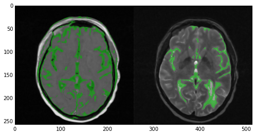
Now take a look at the results of the segmentation. In the T1 image (left) the algorithm did quite a good job covering the majority of the gray matter. However, multiple areas of the skin and fat were also included. In the case of the T2 image (right) the results were nowhere near as good. Multiple areas of gray matter were not segmented despite the large number of iterations. You can experiment with the numberOfIterations and multiplier parameters if you want but chances are you’ll end up segmenting the entire head. Alternatively you can apply more stringent criteria and up the number of seed points. However, here’s where multi-modal segmentation comes into play.

Multi-Modal Segmentation

As discussed, multi-modal segmentation gives us multiple views of the same anatomies. In our case by combining the T1 and T2 images we get two significantly different views of the gray matter and areas that were not connected in one of the images may be connected in the other. In addition, specious connections appearing in one image due to excessive noise or artifacts will most likely not appear in the other.

This allows us to perform the segmentation having more information in our arsenal and achieving the same or better results with more stringent criteria and far fewer iterations. Let’s see the code:

imgComp = SimpleITK.Compose(imgT1Smooth, imgT2Smooth)

imgGrayMatterComp = SimpleITK.VectorConfidenceConnected(image1=imgComp, 
                                               seedList=lstSeeds,
                                               numberOfIterations=1,
                                               multiplier=0.1,
                                               replaceValue=labelGrayMatter)

sitk_show(SimpleITK.LabelOverlay(imgT2SmoothInt[:,:,idxSlice], 
                                 imgGrayMatterComp[:,:,idxSlice]))

Firstly, we begin by ‘combining’ the two images. In order to do that we simply use the ComposeImageFilter which we also used in the sitk_tile_vec auxiliary function. Through that filter we create a single multi-component image containing the information of both T1 and T2 images. The result of the composition is the imgComp image.

Then all we need to do is perform the segmentation. However, as you see in the above code, we don’t just use the ConfidenceConnectedImageFilter class but rather the VectorConfidenceConnectedImageFilter class. The mechanics are exactly the same with the pivotal difference being that VectorConfidenceConnectedImageFilter performs the operation on a vector image, i.e., an image with multiple components per pixel (as is our case).

Note that we’re using the same seeds but much more stringent criteria, i.e., low multiplier value, and only 1 iteration! The result can be seen below:

As you can see, the results are quite great. Not only did we get rid of the skin and fat parts that segmentation on the T1 image gave us, but we also segmented pretty much all gray matter! Of course the segmentation is not perfect as multiple areas of white matter are also segmented but given our lazy approach they’re pretty decent.

Finally, we can store the results of our segmentation as a separate .mhd file containing only the gray matter label. As we saw when loading the input .mhd files, SimpleITK makes these type of operation ridiculously easy. In order to save imgGrayMatterComp under the filename GrayMatter.mhd all we need to do is the following:

SimpleITK.WriteImage(imgGrayMatterComp, "GrayMatter.mhd")

You can download the .mhd and accompanying .raw directly from the Bitbucket repo of this blog. Now we can open this file with any of the software supporting the MHD format. In our case I opened it in ParaView and used the built-in Contour filter to get a 3D iso-surface of our segmentation which you can see in the next figure.

Links & Resources

Material

Here’s the material used in this post:

• IPython Notebook showing the presented process.
• MRI Dataset of a patient’s anatomy acquired with T1 and T2 weighting.
• Gray Matter Segmentation: the .mhd and accompanying .raw file containing the results of the segmentation.

See also

Check out these past posts which were used and referenced today or are relevant to this post:

• IPython Notebook & VTK
• NumPy to VTK: Converting your NumPy arrays to VTK arrays and files
• DICOM in Python: Importing medical image data into NumPy with PyDICOM and VTK
• Surface Extraction: Creating a mesh from pixel-data using Python and VTK
• Image Segmentation with Python and SimpleITK

Don’t forget: all material I’m presenting in this blog can be found under the PyScience BitBucket repository.